Normality Tests

Theoretical Context

In many cases, data follows a normal (Gaussian) distribution or is assumed to do so. Can we use statistical methods to verify that the data at hand is indeed drawn from a normal distribution? Such methods are commonly referred to a normality tests and come in a variety of forms and complexity. Here, we will summarize a number of them in order of increasing sophistication and apply them to an explicit example.

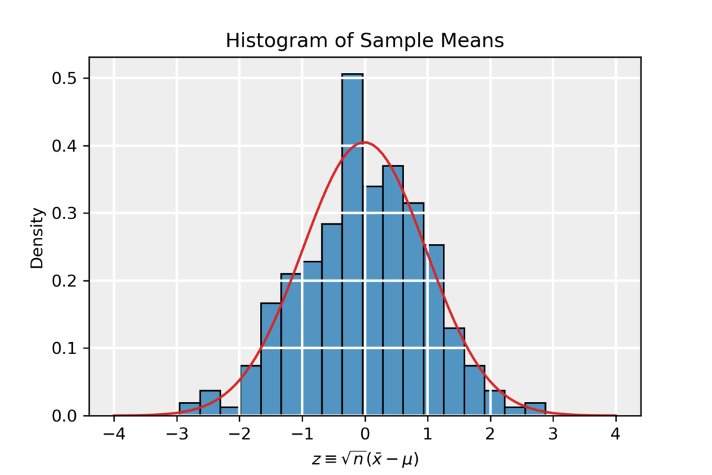
The example we will use stems from the page on the Central Limit Theorem. The distribution of averages of samples drawn from the exponential distribution follows a normal distribution in the limit where the sample size becomes large (n\to \infty) as dictated by the CLT (see the page on the CLT for more details). Hence, this data is perfectly suitable as a test case for normality tests. We work with the renormalized data z\equiv \sqrt{n}(\bar{x}-\mu) and the corresponding histogram is shown below.

1. Skewness and Kurtosis

The first test for normality has been discussed on the page on the Central Limit Theorem as well. A normal distribution has zero skewness g_1 and (excess) kurtosis g_2. Estimating the skewness and kurtosis from the data allows to test for normality. Estimates \hat{g}_{1,2} close to zero suggest a normal distribution.

Using the method of moments, the estimates can be obtained using the moments of the sample:

\begin{equation*}
\hat{g}_1=\frac{m_3}{m_2^{3/2}},\quad\quad\quad \hat{g}_2=\frac{m_4}{m_2^2}-3,
\end{equation*}

where the moment m_r of a dataset is given by:

\begin{equation*}
m_r=\frac{1}{n}\sum_{i=1}^n (x_i-\bar{x})^r,
\end{equation*}

where \bar{x} is the sample average. The errors in the estimate depend solely on the sample size n and read:

\begin{align*}
\sigma^2_{\hat{g}_1} &= \frac{6n(n-1)}{(n-2)(n+1)(n+3)}\to\frac{6}{n}, \\
\sigma^2_{\hat{g}_2} &= \frac{4(n^2-1)}{(n-3)(n+5)} \sigma^2_{\hat{g}_1} \to \frac{24}{n},
\end{align*}

where the asymptotes apply in the range of large sample size n.

The estimates where found to be \hat{g}_1=-0.12\pm0.11 and \hat{g}_2=0.020\pm0.010, which are in agreement with the assumption of normality.

2. P-P Plot

Given two cumulative density functions (CDFs) F_{0,1} (e.g. one empirical CDF and one theoretical CDF), plot them against each other. If the two CDFs are identical, the obtained plot concides with the straight line from (0,0) to (1,1).

To illustrate this method, we take F_0 to be the hypothesized distribution of the example data, corresponding to a normal with average zero and unit variance. The CDF is then:

\begin{equation*}
F_0=\frac{1}{2}\bigg[1+\mathrm{erf}\big(x/\sqrt{2}\big)\bigg],\quad\quad\quad \mathrm{erf}(z)\equiv \frac{2}{\sqrt{\pi}}\int_{-\infty}^z e^{-t^2}\;dt.  
\end{equation*}

As F_1 we take the empirical CDF F_n as obtained from the data:

\begin{equation*}
F_n(x) = \frac{\mathrm{number\;of\;elements\;in\;sample}\leq x}{n}. 
\end{equation*}

Below, we present the P-P plot for the example data, we see that the data follows the diagonal to reasonably well, suggesting that the data follows CDF F_0 and is therefore normally distributed. More precisely, the P-P plot suggests that the empirical CDF approaches the theoretical distribution in the limit of infinite sample size:

\begin{equation*}
\lim_{n\to\infty} F_n(x)=F_0(x). 
\end{equation*}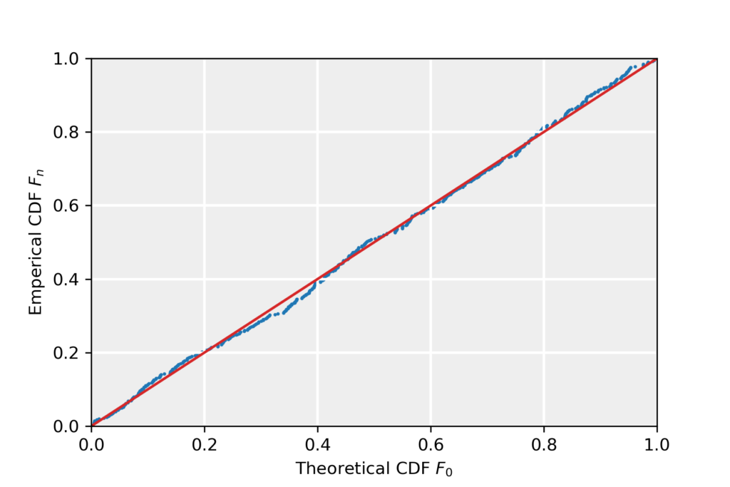

3. Confidence Bands on Empirical CDF

The Drovetsky-Kiefer-Wolfowitz inequality states that the true CDF F_0 from which a data sample is drawn is contained, with probability or confidence level (CL) 1-\alpha, in the interval:

\begin{equation*}
F_n(x)-\varepsilon\leq F_0(x)\leq F_n(x)+\varepsilon,
\end{equation*}

where F_n(x) is the empirical CDF for sample size n and the parameter is given by:

\begin{equation*}
\varepsilon\equiv \sqrt{\ln(2/\alpha)/2n}. 
\end{equation*}

The inequality above defines a confidence band around the empirical CDF. The hypothesized CDF F_0 being contained within this band suggests that it described the data at CL of 1-\alpha.

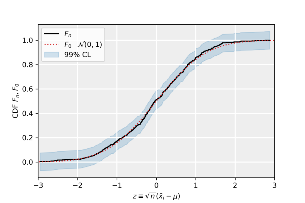
For our example data, we have taken \alpha=0.01 corresponding to a confidence level of 99%. We have plotted the empirical distribution in black, the theoretical CDF F_0 corresponding to a normal distribution (defined above in terms of the error function) in dotted red. The confidence band is denoted in light blue. Since the theoretical CDF is well contained in this band, at 99% CL we accept F_0.

4. Kolmogorov-Smirnov (KS) Test

The KS test is a non-parametric test of equality of continuous one-dimensional distributions that can be used to compare a sample with a reference probability distribution. Let the sample \{x_1,x_2,\dots,x_n\} be drawn from an unknown CDF F(x) and take F_0 to be the hypothesized CDF. The KS test tests the null hypothesis against the alternative hypothesis:

\begin{align*}
H_0&:F(x)=F_0(x),\\
H_a&:F(x)\neq F_0(x).
\end{align*}

The test statistic D_n is defined as:

\begin{equation*}
D_n=\sup_{x\in\mathbb{R}}|F_n(x)-F_0(x)|.
\end{equation*}

In other words, the test statistic takes the largest difference (supremum) between the empirical CDF and the hypothesized CDF. Under the null hypothesis, i.e. assuming F(x)=F_0(x), the normalized statistic K\equiv \sqrt{n}D_n follows the Kolmogorov distribution as n\to\infty. In practice, the Kolmogorov distribution is a good approximation to the distribution of the test statistics for n\gtrsim 100. The Kolmogorov CDF is given by:

\begin{align*}
F_K(x)&\equiv \mathrm{P}(K\leq x) \\
&= 1-2\sum_{k=1}^{\infty}(-1)^{k-1}\;e^{-2k^2x^2}. 
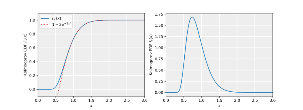
\end{align*}

For x>1, we can employ the approximation F_K(x)\simeq 1-2e^{-2x^2}. In the figure below, we numerically evaluated the Kolmogorov distribution by taking into account the first 10^5 terms in the sum (blue curve) and show the approximation (red dotted curve). In the right panel, we show the probability density function f_K(x)=\partial_x F_K(x).

At significance level \alpha, we defined the critical value K_\alpha via:

\begin{equation*}
F_K(K_\alpha)=\mathrm{P}(K\leq K_\alpha)=1-\alpha.
\end{equation*}

In case the test statistic is smaller than the critical value, i.e. K\leq K_\alpha, we do not reject the null hypothesis at significance level \alpha. Otherwise we reject the null hypothesis. In case K_\alpha>1, we can find an analytic expression by using the approximation for Kolmogorov’s CDF and solving for the critical value:

\begin{equation*}
F_K(K_\alpha)\simeq 1-2e^{-2K_\alpha^2}=1-\alpha\quad\to\quad K_\alpha=\sqrt{\frac{-\ln(\alpha/2)}{2}}. 
\end{equation*}

For the example data, we take the hypothesized distribution F_0 to be corresponding to a normal distribution with zero mean and unit variance (as defined with the P-P plot as well). The rescaled test statistic is found to be K=0.709. The critical value at significance level \alpha=0.01 is K_{\alpha=0.01}=1.628, so we do not reject the null hypothesis. Therefore, the KS test suggests that the data is normally distributed.

Downloads