Kepler’s Laws

Animations

Theoretical Context

Kepler’s laws are most often presented in a form applicable when one of the two bodies, the primary (mass M), is much heavier than the orbiting body, the satellite (mass m). However, the most general form of Kepler’s laws still applies when this mass hierarchy (where m\ll M) is not enforced. The scenario where we have two bodies with arbitrary masses m_{1,2} interacting gravitationally is known as the two-body problem. In the simulations presented here, the general two-body problem is solved numerically, after which the familiar mass hierarchy is enforced only is certain examples.

Reduction to Two One-Body Problems

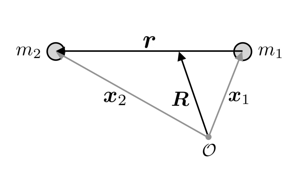
Let the two masses m_{1,2} be located at positions \boldsymbol{x}_{1,2} relative to the origin \mathcal{O}. We denote by \boldsymbol{F}_{ij} the gravitational force on the i-th body due to the j-th body:

\begin{equation*}
\boldsymbol{F}_{ij} = -Gm_im_j\frac{\boldsymbol{r}_{ij}}{r_{ij}^3},
\end{equation*}

where \boldsymbol{r}_{ij}\equiv \boldsymbol{x}_i-\boldsymbol{x}_j. In this notation, note that \boldsymbol{F}_{12} is the gravitational force on body 1 due to body 2. Note furthermore that \boldsymbol{F}_{12}=-\boldsymbol{F}_{21} since \boldsymbol{r}_{12}=-\boldsymbol{r}_{21}, this is a simple consequence of Newton’s 3rd law.

The equations of motion for the two masses reads:

\begin{equation*}
m_1\ddot{\boldsymbol{x}}_1 = \boldsymbol{F}_{12},\quad\quad\quad m_2\ddot{x}_2 = \boldsymbol{F}_{21}.
\end{equation*}

In the current form of the system of equations is not convenient to solve. Instead, we will recast the problem in terms of a coordinate (\boldsymbol{R}) describing the motion of the center of mass (the barycenter) and one (\boldsymbol{r}) describing the motion of body 2 relative to body 1:

\begin{equation*}
\boldsymbol{R}\equiv \frac{m_1\boldsymbol{x}_1+m_2\boldsymbol{x}_2}{m_1+m_2},\quad\quad\quad \boldsymbol{r}\equiv\boldsymbol{r}_{12}=\boldsymbol{x}_1-\boldsymbol{x}_2. 
\end{equation*}

Adding the equations of motion we find:

\begin{equation*}
m_1\ddot{\boldsymbol{x}}_1+m_2\ddot{\boldsymbol{x}}_2 = (m_1+m_2)\ddot{\boldsymbol{R}} = \boldsymbol{F}_{12}+\boldsymbol{F}_{21}=0,
\end{equation*}

implying that \ddot{\boldsymbol{R}}=0, i.e. the center of mass does moves at a constant velocity. Without loss of generality, we take the center of mass to be stationary at the origin, i.e. \boldsymbol{R}=0. Subtracting gives:

\begin{equation*}
\ddot{\boldsymbol{r}}=\ddot{\boldsymbol{x}}_1-\ddot{\boldsymbol{x}}_2 = \frac{\boldsymbol{F}_{12}}{m_1}-\frac{\boldsymbol{F}_{21}}{m_2}=\frac{\boldsymbol{F}_{12}}{m_\mathrm{R}},\quad\quad\quad m_\mathrm{R}\equiv\frac{m_1m_2}{m_1+m_2},
\end{equation*}

where m_\mathrm{R} is the reduced mass. Substituting the expression for the gravitational force \boldsymbol{F}_{21}, we get:

\begin{equation*}
\ddot{\boldsymbol{r}}=-\mu\frac{\boldsymbol{r}}{r^3},
\end{equation*}

in which \mu\equiv G(m_1+m_2). Note that we now have two independent equations of motion for \boldsymbol{R} and \boldsymbol{r}. That is, we reduced the two-body problem to two independent one-body problems. The solutions to \boldsymbol{x}_{1,2} can then be obtained from \boldsymbol{R} and \boldsymbol{r} as:

\begin{equation*}
\boldsymbol{x}_1=\boldsymbol{R}+\frac{m_2}{m_1+m_2}\boldsymbol{r},\quad\quad\quad \boldsymbol{x}_2=\boldsymbol{R}-\frac{m_1}{m_1+m_2}\boldsymbol{r}.
\end{equation*}

In the center of mass frame, the bodies trace out ellipses with one of their foci at located at the center of mass, as visible in the CM animation at the top of this page.

Physical Interpretation

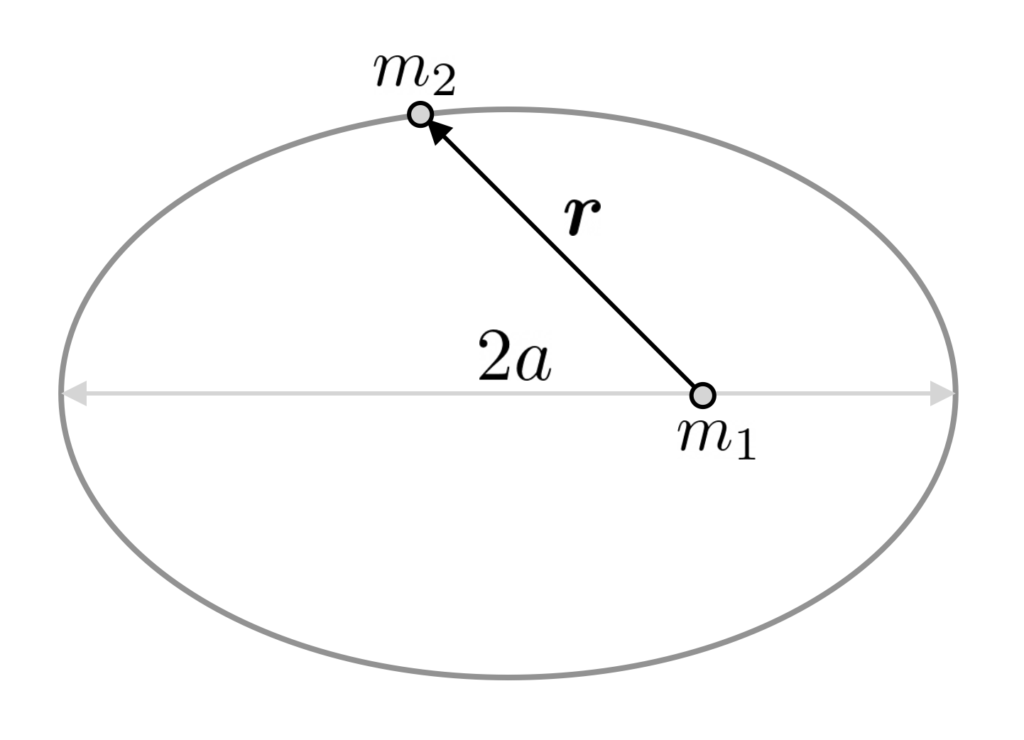
Upon solving Eq. 6, one finds that \boldsymbol{r}(t) traces out an elliptical orbit: this is Kepler’s first law. More precisely, in the rest frame of m_2, m_1 follows an elliptical orbit with m_2 located at a focus of the ellipse. The orbital period T of the ellipse is directly related to the semi-major axis a as:

\begin{equation*}
T^2=\frac{4\pi^2}{\mu}a^3,
\end{equation*}

implying that orbits with the same semi-major axis have the same orbital period. At any point along the orbit, the speed of the orbiting body (i.e. m_2) is given by:

\begin{equation*}
v^2=\mu\Big(\frac{2}{r}-\frac{1}{a}\Big).
\end{equation*}

In the simulations, the initial conditions are set at the point of closest approach, corresponding to r_c=a(1-\epsilon), where \epsilon is the eccentricity. At that point, the velocity vector is always perpendicular to the position vector and its magnitude is given by:

\begin{equation*}
v_c=\sqrt{\frac{\mu}{a}\frac{1+\epsilon}{1-\epsilon}}. 
\end{equation*}

Reduction to Primary-Satellite System

So far, we have take the masses of the body to be arbitrary, and their effect enters the equations via the parameter \mu\equiv G(m_1+m_2). Let us take m_1\equiv M and m_2\equiv m with the additional constraint that M\gg m so that \mu=GM up to corrections of order \mathcal{O}(m/M). That is, M is the primary and m is the satellite. In this limit, we find for the center of mass:

\begin{equation*}
\boldsymbol{R}=\frac{M}{M+m}\boldsymbol{x}_1+\frac{m}{M+m}\boldsymbol{x}_2\simeq \boldsymbol{x}_1+\mathcal{O}(m/M),
\end{equation*}

so that the center of mass is essentially identical to the located of the primary. Without loss of generality, we can then take the stationary location of the primary to be at the origin.

Kepler formulated his famous laws of planetary motion in this setup, where the sun is the primary and the planet acts as the satellite:

1. The orbit of a planet is an ellipse with the sun at one of the two foci.
2. A line segment joining the planet and the sun sweeps out equal areas in equal time intervals.
3. The square of the planet’s orbital period is proportional to the cube of the semi-major axis of the orbit.

Kepler’s laws are illustrated by the animations on the top of this page (indicated by K1, K2, K3).

Downloads