Theoretical Context
In data analysis, we have a data sample drawn from a distribution with unknown parameters and we wish to estimate these parameters from the sample. A well known method to do this is the so-called maximum likelihood method.
Suppose that the random variables \{X_1,\dots, X_n\} have a joint probability density function f(x_1,\dots, x_n|\theta) depending on a parameter \theta. This is the probability of observing data values X_i=x_i\;(I=1,\dots,n) given the parameter \theta, commonly referred to as the likelihood:
\begin{equation*}
\mathcal{L}(\theta)\equiv f(x_1,\dots,x_n|\theta).
\end{equation*}
As the notation suggests, we regard the likelihood as a function of the parameter. The analysis below easily extends to distributions multiple parameters \theta_i. The maximum likelihood estimate (MLE) \hat{\theta}_{\mathrm{MLE}} is that value of \theta that maximizes the likelihood. In other words, the estimate gives the value of \theta that makes the observed data most probable (read likeli) given the assumed distribution.
Assuming X_i are identical independently distributed (i.i.d.) random variables, the joint probability is the product of the probability density function for the individual data f(x_i|\theta):
\begin{equation*}
\mathcal{L}(\theta)=\prod_{i=1}^n f(x_i|\theta).
\end{equation*}
We then maximize the likelihood to find the MLE. Numerically, however, it is most often easier to maximize the logarithm of the likelihood \ell(\theta)\equiv\ln\mathcal{L}(\theta), which gives the same result as the logarithm is a monotonic function. This has the convenient property that we get sums instead of products:
\begin{equation*}
\ell(\theta)=\sum_{i=1}^n\ln f(x_i|\theta).
\end{equation*}
Hence, MLE estimate is found by solving:
\begin{equation*}
\frac{\partial}{\partial\theta} \ell(\theta)\bigg|_{\theta=\hat{\theta}_\mathrm{MLE}}=0.
\end{equation*}
Consistency and Sampling Distribution
In the limit of large samples (formally, when n\to\infty), we can derive the sampling distribution of the MLE estimators and show that hey are consistent. We will not give a rigorous treatment here. Instead, we justify our approach in a simplified context.
Consistency MLE Estimate: In the limit of large sample size n, the estimator \hat{\theta}_\mathrm{MLE} is consistent for an i.i.d. sample drawn from a distribution that is smooth (continuous).
We sketch the proof for this statement below. Note that maximizing \ell(\theta) with respect to \theta is equivalent to maximizing S_n(\theta)\equiv \ell(\theta)/n. In the limit n\to\infty, the law of large numbers dictates:
\begin{equation*}
\lim_{n\to\infty} S_n(\theta)=\int dx\;\ln f(x|\theta)\;f(x|\theta_0)=\mathbb{E}[\ln f(x|\theta)]\equiv S(\theta),
\end{equation*}
where \theta_0 denotes the true parameter of the distribution. In other words, for large samples, the estimate \hat{\theta}_\mathrm{MLE} maximizing \ell(\theta) approaches the value that maximizes S(\theta). Maximizing the latter, we get:
\begin{equation*}
\frac{\partial S}{\partial \theta}=\int dx\;\frac{\partial f(x|\theta)}{\partial\theta}\;\frac{f(x|\theta)}{f(x|\theta_0)}.
\end{equation*}
We proceed by showing that \theta=\theta_0 is a stationary point of S as follows:
\begin{equation*}
\frac{\partial S}{\partial \theta}\bigg|_{\theta=\theta_0}=\int dx\;\frac{\partial f(x|\theta)}{\partial\theta} = \frac{\partial}{\partial\theta}\int dx\;f(x|\theta)=\frac{\partial}{\partial\theta}(1)=0.
\end{equation*}
Showing that the stationary point is indeed a maximum is not trivial. The following serves as an heuristic argument. We assume that \ell(\theta) increases continuously towards the maximum value when approaching from the left (\theta\to\theta_0^-) as well as from approaching from the right (\theta\to\theta_0^+), so that:
\begin{equation}
\ell'(\theta)\big|_{\theta<\theta_0}>0,\quad\quad\quad \ell'(\theta)|_{\theta>\theta_0}<0,
\end{equation}
suggesting that \ell(\theta_0) is indeed a maximum.
Consistency is established as follows. In the large sample limit we have:
\begin{equation*}
\lim_{n\to\infty}S_n(\theta)=S(\theta).
\end{equation*}
Taking the derivative with respect to \theta gives:
\begin{equation*}
\lim_{n\to\infty} \frac{\partial S_n}{\partial\theta}=\frac{\partial S}{\partial\theta}.
\end{equation*}
Technically, taking the derivative of the limiting behavior above require that S_n is uniformly convergent. Evaluating at \theta=\theta_0, we have:
\begin{equation*}
\lim_{n\to\infty} \frac{\partial S_n}{\partial\theta}\bigg|_{\theta=\theta_0}=\frac{\partial S}{\partial\theta}\bigg|_{\theta=\theta_0}=0.
\end{equation*}
Now, recall that we find the MLE estimate by requiring \partial S_n/\partial\theta to vanish. Hence, for large samples we expect that \hat{\theta}_{\mathrm{MLE}}\to\theta_0 and the MLE estimate is consistent.
Now we turn to the sampling distribution. In the large sample limit, the sample distribution f_\Theta(\theta) is normal with mean \theta_0 and variance 1/nI(\theta_0), where:
\begin{equation*}
I(\theta)=-\mathbb{E}\bigg[\frac{\partial^2}{\partial\theta^2}\ln f(x|\theta)\bigg].
\end{equation*}
As you might expect, the reason for normality of the sampling distribution is the Central Limit Theorem. For a more rigorous proof, see e.g. Mathematical Statistics and Data Analysis by John A. Rice, section 8.5.2.
Example
Consider the exponential distribution, whose probability density function is given by f(x|\lambda)=\lambda e^{-\lambda x}. We assume we have independent results x_i\;(i=1,\dots, n). The log-likelihood is then:
\begin{equation*}
\ell(\lambda)= n\ln(\lambda)-n\lambda\;\bar{X}.
\end{equation*}
Taking the derivative with respect to \lambda gives:
\begin{equation*}
\frac{\partial \ell}{\partial \lambda}\bigg|_{\lambda=\hat{\lambda}_\mathrm{MLE}}=n\bigg[\frac{1}{\hat{\lambda}_\mathrm{MLE}}-\bar{X}\bigg]=0, \quad\quad\quad \hat{\lambda}_\mathrm{MLE}=\frac{1}{\bar{X}}.
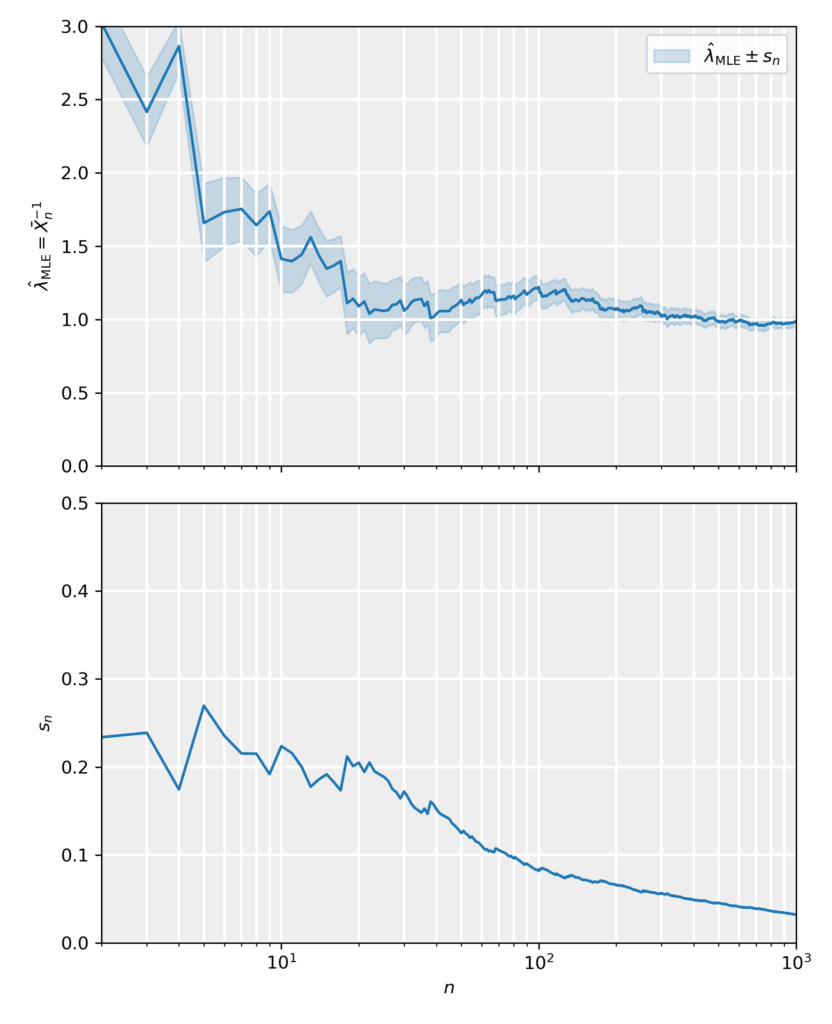
\end{equation*}In this case, the estimate is equivalent to that obtained using the Method of Moments (recall that \lambda=\beta^{-1}). This is often the case, although we will consider examples in which the MME and MLE estimates differ. For the function I we found I(\lambda)=1/\lambda^2 so that the variance and standard error are given by:
\begin{equation*}
\sigma^2_{\hat{\lambda}_\mathrm{MLE}}=\frac{1}{n\lambda^2},\quad\quad\quad s_{\hat{\lambda}_\mathrm{MLE}}=\frac{1}{\hat{\lambda}_\mathrm{MLE}\sqrt{n}}=\frac{\bar{X}}{\sqrt{n}},
\end{equation*}
which are again in agreement with the MME estimates. In the figure and attached notebook, we have generated data samples from an exponential distribution with rate parameter \lambda=1 and sizes in the range n\in[1,10^3]. For those data samples we have calculated the MLE estimates and standard errors, and plotted them as a function of the sample size. The results show that the MLE estimate is consistent estimate, as it tends towards the true value in an unbiased fashion and its error approaches zero accordingly.