Magnet Falling Through Copper Pipe

Physical Interpretation

When a magnet falls through a copper pipe, something remarkable happens: it appears to fall in slow-motion. The reason for the slower movement of the magnet inside the pipe is the generation of Eddy currents and the associated magnetic damping force. Imagine a small ring that is part of the overall pipe. As the magnet approaches the ring (from above), the flux through the ring increases. On account of Lenz’ law, a current in the ring and associated magnetic field will be induced so as to oppose the change in flux. The induced magnetic field in the ring causes an upward drag force on the magnet, causing it to fall slower than it would in free-fall.

Description of the Applet

The mathematica notebook (to be downloaded at the bottom of the page) contains an applet that allows you to change various characteristics of the system, such as the magnet strength and the pipe radius and thickness. In varying these parameters you can develop an intuition for the characteristic behavior of the system. The applet contain the following panels:

• Left Panel: Shows the pipe and magnet. You can think of the pipe as comprised of rings stacked on top of each other. Three such rings are highlighted in red, green and blue. The arrow shows the direction of current flow in those rings. Notice that as the magnet passes the ring, the direction changes. The upward arrows on each rings indicate the direction and magnitude of the repulsive force acting on the dipole due to the respective ring.
• Top Right Panel: Shows characteristics of the rings: you can chose between the flux through the ring, the electromotive force (voltage) in the ring, or the current flowing in the ring. These quantities are plotted against the vertical separation between the ring (located at z_r) and the magnet z_d. The colored dots represent the corresponding rings. For instance, as the magnet approaches the red ring, the flux increases and reaches a maximum as the magnet perfectly aligned inside the magnet.
• Middle Right Panel: Shows the force on each ring as function of separation between the rings and the magnet.
• Lower Right Panel: Plots the vertical postion of the dipole as a function of time (solid line). The dotted line represents the asymptotic behavior of the magnet as it reaches its terminal velocity.

Theoretical Background

Here, we will examine the motion of the magnet through the copper pipe in a quantitative manner. We will approach the problem as follows. We divide the pipe into infinitesimal conducting rings and calculate the infinitesimal element of force that each ring exerts on the magnet. Summing (i.e. integrating) over all these rings, we obtain the combined force on the magnet due to the entire pipe.

Magnetic Dipole Approximation

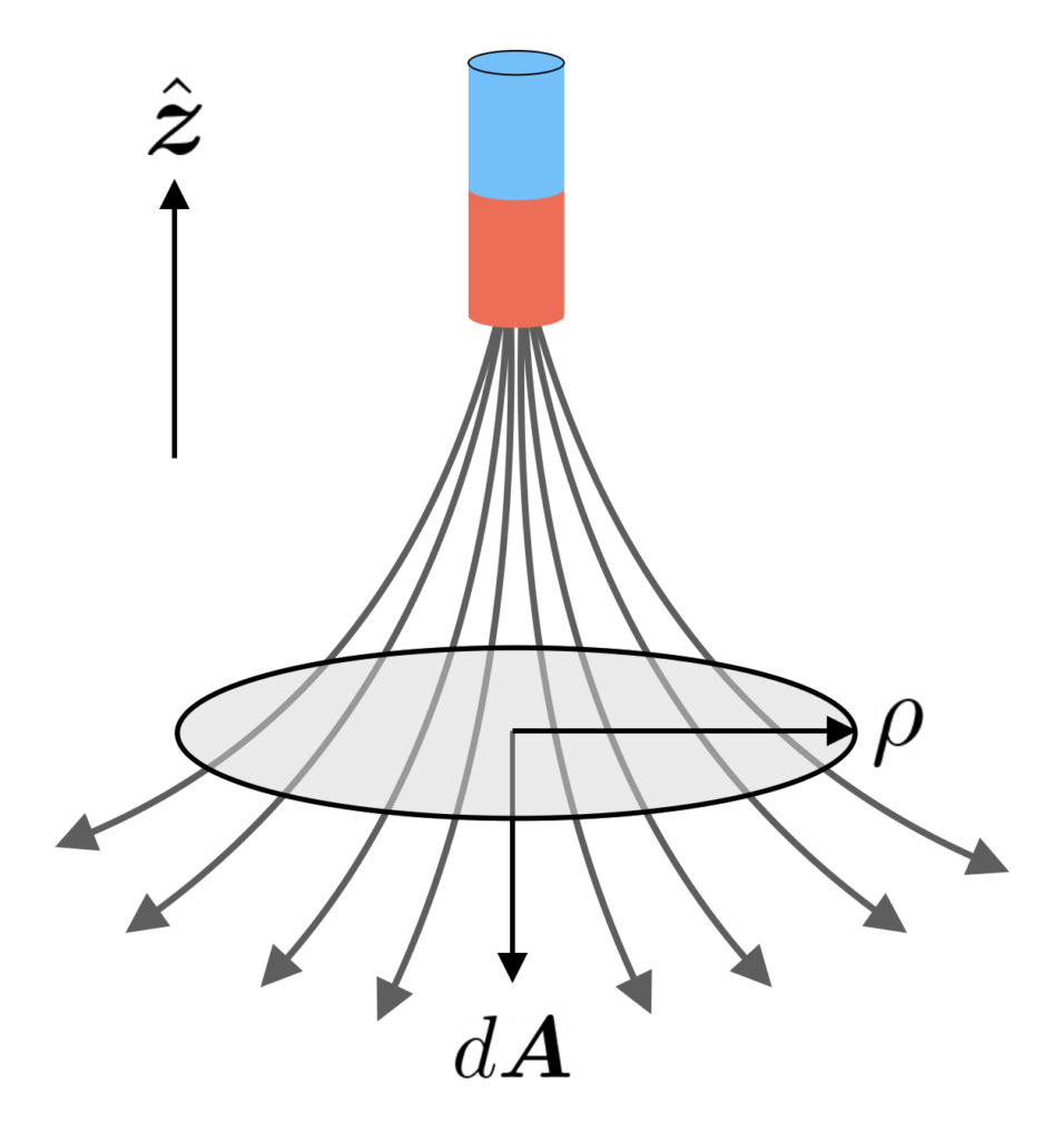
To simplify the analysis, we model the magnet as being a magnetic dipole with magnetic moment M. We use cylindrical coordinates (\hat{\boldsymbol{z}},\hat{\boldsymbol{\rho}},\hat{\boldsymbol{\phi}}) and assume that the North Pole of magnet points down, i.e. the magnetization is \boldsymbol{m}=-M\hat{\boldsymbol{z}}. We write the dipole field as:

\begin{equation*}
\boldsymbol{B}_\mathrm{dip}=B_z\hat{\boldsymbol{z}}+B_\rho\hat{\boldsymbol{\rho}},
\end{equation*}

where we excluded the angular component as it vanishes by cylindrical symmetry. The other two components read:

\begin{align*}
B_z&=-\mu\bigg[\frac{3z^2}{(\rho^2+z^2)^{5/2}}-\frac{1}{(\rho^2+z^2)^{3/2}}\bigg],\\
B_\rho &=+\mu\frac{3z\rho}{(\rho^2+z^2)^{5/2}},
\end{align*}

where we have defined \mu\equiv\mu_0 M/4\pi.

Flux and EMF

We now compute the flux through a ring of radius \rho located at the origin (z=0) due to a dipole located at a height z. The infinitesimal area element is d\boldsymbol{A}=-2\pi\rho\;d\rho\;\hat{\boldsymbol{z}}, so that the flux becomes:

\begin{equation*}
\Phi_B=\int \boldsymbol{B}\cdot d\boldsymbol{A}=\int B_z(\rho)\;dA_z(\rho)=2\pi \mu\;\frac{\rho^2}{(\rho^2+z^2)^{3/2}}. 
\end{equation*}

Note that the flux increases as the distance between the ring and the dipole decreases, reaches a maximum when the dipole is vertically aligned with the ring, and decreases again when the exits the ring.

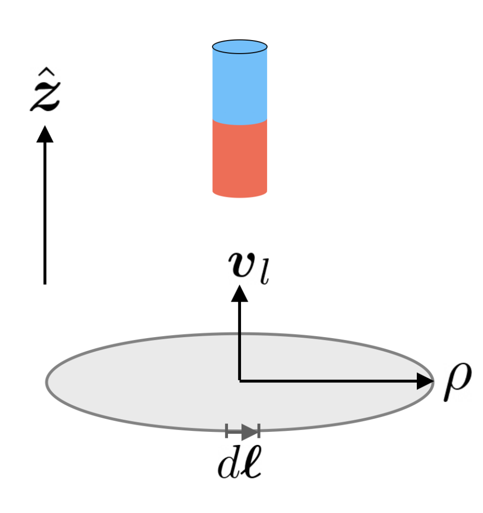
Now that we have computed the flux, we proceed with the EMF. The schematic used for this calculation is shown in the right image above. The vertical distance between the loop and the dipole is still z. The EMF generated in a loop moving with a velocity \boldsymbol{v}_l with respect to a magnetic field \boldsymbol{B} is:

\begin{equation*}
\varepsilon=\int_\mathrm{loop} (\boldsymbol{v}_l\times \boldsymbol{B})\cdot d\boldsymbol{\ell},
\end{equation*}

where d\boldsymbol{\ell} is the infinitesimal line element along the considered loop. Since the dipole falls in the negative z direction, i.e. \boldsymbol{v}_d=-v_d\hat{\boldsymbol{z}} with v_d>0, in the rest frame of the dipole, the loop moves at velocity \boldsymbol{v}_l=v_d\hat{\boldsymbol{z}}. The cross product then becomes:

\begin{equation*}
\boldsymbol{v}_l\times \boldsymbol{B}=v_dB_\rho\;\hat{\boldsymbol{\phi}}. 
\end{equation*}

Given that the line element is d\boldsymbol{\ell}=\rho\;d\phi\;\hat{\boldsymbol{\phi}} yields:

\begin{equation*}
\varepsilon=\int (\boldsymbol{v}_l\times \boldsymbol{B})\cdot d\boldsymbol{\ell}=v_dB_\rho\;\rho\int_0^{2\pi}d\phi=2\pi\rho\;v_dB_\rho,
\end{equation*}

for the induced EMF.

Force due to Ring

Given the EMF, we are now in the position to derive the force the ring exerts on the dipole. By Newton’s third law, the force on the magnet by the ring is the negative of that on the ring due to magnet. We denote by d\boldsymbol{F}_\mathrm{ring-mag} the force exerted by the dipole on a chunk of ring with length d\boldsymbol{\ell} containing a current dI:

\begin{equation*}
d\boldsymbol{F}_\mathrm{ring-mag}=dI(d\boldsymbol{\ell}\times \boldsymbol{B}_\mathrm{dip}). 
\end{equation*}

The force on the dipole magnet is then:

\begin{equation*}
\boldsymbol{F}_\mathrm{mag-ring}=-\int d\boldsymbol{F}_\mathrm{ring-mag}=-\int dI(d\boldsymbol{\ell}\times \boldsymbol{B}_\mathrm{dip}),
\end{equation*}

in which the cross product becomes:

\begin{equation*}
d\boldsymbol{\ell}\times \boldsymbol{B}_\mathrm{dip}=B_z\rho\;d\phi\;\hat{\boldsymbol{\rho}}-B_\rho\rho\;d\phi\;\hat{\boldsymbol{z}}.
\end{equation*}

Integrating over the total ring then gives:

\begin{equation*}
\boldsymbol{F}_\mathrm{mag-ring}=\int dI\;\rho\big(-B_z\;d\phi\;\hat{\boldsymbol{\rho}}+B_\rho\;d\phi
\;\hat{\boldsymbol{z}}\big)
\end{equation*}

In the above equation, we did not express the current in the loop dI in terms of the EMF. Below, we will do this for an infinitesimally thin ring of width d\rho and height dz, centered around coordinates (\rho,z) as indicated in the picture below.

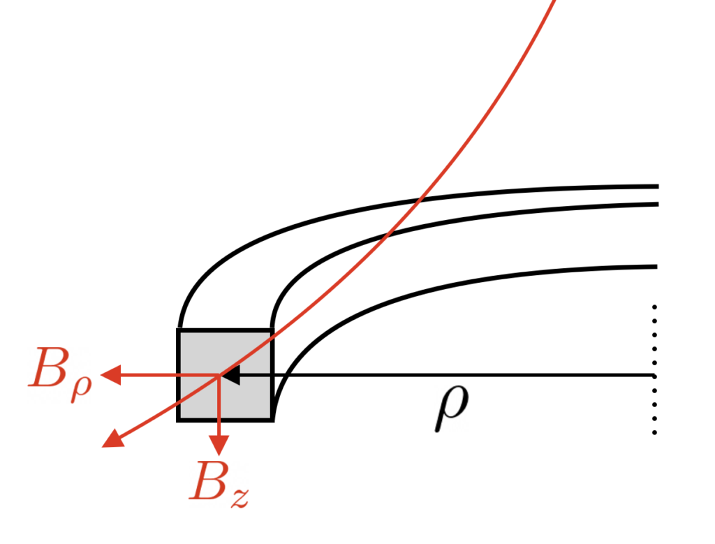
The current running in the ring of radius \rho is denoted as dI, which can be related to the EMF as dI=\varepsilon(\rho)\;dC. Here, dC is the differential conductance in the ring (the reciprocal of the restitance). Given the length (circumference) of the ring 2\pi\rho, its cross section dA=d\rho\;dz and the conductivity \sigma, we have:

\begin{equation*}
dC=\frac{\sigma}{2\pi\rho}\;d\rho\;dz.
\end{equation*}

Plugging in the EMF for a ring of radius \rho, we get the following expression for the differential current:

\begin{equation*}
dI=\sigma v_d\;B_\rho\;d\rho\;dz. 
\end{equation*}

Finally, we find the following expression for the force between the on the magnet due to the ring:

\begin{equation*}
\boldsymbol{F}_\mathrm{mag-ring}=\sigma v_d\int\big(-B_zB_\rho\;\hat{\boldsymbol{\rho}}+B_\rho^2\;\hat{\boldsymbol{z}}\big)\;dV,
\end{equation*}

where dV=\rho\;d\rho\;dz\;d\phi is the volume element in cylindrical coordinates. In case we want the force due to a single ring, we solely integrate over \phi, and assume that B_\rho and B_z are constant across the cross section dA=d\rho\;dz. Below, we will integrate over the entire volume of the pipe, i.e. stacking rings on top of each other to form a tube, to obtain the total force on the magnet due to the pipe.

Force due Entire Pipe

To obtain the total force on the magnet, \boldsymbol{F}_\mathrm{mag-pipe}, we integrate over the volume of the pipe. We assume the pipe is very long so that we can integrate z over the interval (-\infty, +\infty). We integrate \rho over the range [a,b], the inner and outer radius of the pipe. Note that the product B_zB_\rho is odd in z, so that the associated integral vanishes and we are left with the integral:

\begin{equation*}
\boldsymbol{F}_\mathrm{mag-ring}=\sigma v_d\int B_\rho^2\;dV\;\hat{\boldsymbol{z}},
\end{equation*}

which indicates that the force on the magnet is entirely in the z direction. To evaluate the integral, we plug in the expression for B_\rho, yielding:

\begin{equation*}
\boldsymbol{F}_\mathrm{mag-ring}=9\sigma v_d\;\mu^2\int_0^{2\pi}d\phi\int_{a}^bd\rho\int_{-\infty}^{+\infty}dz\;\frac{z^2\rho^3}{(\rho^2+z^2)^5}\;\hat{\boldsymbol{z}}. 
\end{equation*}

The angular integral simply gives 2\pi. The integrals over \rho and z can be disentangled by making introduced the auxiliary variable u\equiv z/\rho, giving:

\begin{equation*}
\boldsymbol{F}_\mathrm{mag-ring}=18\pi\;\sigma v_d\;\mu^2\times\mathcal{I_\rho}\;\mathcal{I}_u\;\hat{\boldsymbol{z}},
\end{equation*}

where the integrals \mathcal{I}_{\rho,u} are defined as:

\begin{align*}
\mathcal{I}_\rho &\equiv \int_a^b\frac{d\rho}{\rho^4} = \frac{1}{3}\bigg[\frac{1}{a^3}-\frac{1}{b^3}\bigg],\\
\mathcal{I}_u &\equiv \int_{-\infty}^{+\infty}du\;\frac{u^2}{(1+u^2)^5}=\frac{5\pi}{256}. 
\end{align*}

Writing the resulting expression in terms of \boldsymbol{v}_d=-v_d\hat{\boldsymbol{z}}, we find that the force on the magnet due to the pipe acts as a drag force of the form:

\begin{equation*}
\boldsymbol{F}_\mathrm{mag-pipe}=-k\boldsymbol{v}_d,\quad\quad\quad k\equiv \frac{30\pi^2}{256}\;\sigma\mu^2\bigg[\frac{1}{a^3}-\frac{1}{b^3}\bigg]= \frac{30\pi^2}{256}\;\frac{\sigma\mu^2}{a^3}\bigg[1-\frac{1}{\lambda^3}\bigg],
\end{equation*}

where we have introduced the thickness parameter \lambda=b/a>1.

Equation of Motion

Assuming the dipole magnet has a mass m, the equation of motion becomes:

\begin{equation*}
m\;\frac{d\boldsymbol{v}_d}{dt}=\boldsymbol{F}_g+\boldsymbol{F}_{\mathrm{mag-pipe}}=-mg\hat{\boldsymbol{z}}-k\boldsymbol{v_d}.
\end{equation*}

In terms of the magnitude v_d, we find:

\begin{equation*}
\frac{dv_d}{dt}=g-\frac{k}{m}v_d. 
\end{equation*}

The solution to the above equation of motion is given by v_d(t)=v_\mathrm{T}(1-e^{-t/\tau}), where the terminal velocity is v_\mathrm{T}\equiv mg/k and the time constant is \tau\equiv m/k. The combined action of retarding (drag) force and gravity results in a short initial transient regime, followed by uniform terminal motion, where the effect of the gravitational and drag force precisely cancel. Assuming a initial position z_0, we find:

\begin{equation*}
z_d(t)=z_0-v_\mathrm{T}\tau\bigg[\frac{t}{\tau}-1+e^{-t/\tau}\bigg]. 
\end{equation*}

Downloads

Unfortunately, the applet is computationally too heavy to work properly in the Wolfram Player, so to run the applet/notebook requires a full version of Wolfram Mathematica.