Tidal Forces

Introduction and Context

The ocean tides are generated by the gravitational forces exerted on the oceans by the moon and the sun. For that reason, they are also called tidal forces. In the video above, we show a simplified animation of the tides generated by the combined gravitational effects of the moon and the sun. For more details on the assumptions and mathematical framework, see the sections below. We consider a frame that co-rotates with the earth and the sun and has its origin at the center of mass of the earth. We assume the moon orbits the earth circularly in the same plane. Furthermore, we assume that the rotation axis of the earth itself is perpendicular to this plane. The earth itself is assumed to be covered completely by ocean, i.e. there are no continents.

The top panel shows a top down view of this simplified system. That is, the equatorial cross section of the earth is shown, surrounded with a layer of ocean and its tidal bulges. The rotating red dot moves corresponds to an observer stationary on the equator. The lower left panel shows the variation in water level for the observer, relative to the water level in case there would be no tidal forces at all. Whenever the moon and the sun are aligned relative to the earth, which happens twice a month, their gravitational effects constructively combine to to cause high tides called spring tides. When they are at right angles, their effects partially cancels and we get lower neap tides. The lower right panel shows a decomposition of the total tidal force into components due to the sun and moon. This panel also shows the constructive and destructive combined effect of the moon and sun at spring and neap tides, respectively.

Assumptions and Approximations

To construct the animation, we have made a number of simplifying assumptions, which will be listed in detail below:

1. Quasi-static Approximation – I

We assume that the oscillation period of the tides T_\mathrm{tid} is small compared to the period of earth’s rotation around its own axis T_\mathrm{R}\sim 1\;\mathrm{day}. In that case, there is enough time for the water surface to reach equilibrium under the combined forces of the earth, moon and sun. We then deal with a simpler statical problem, rather than a dynamical problem. Per day, two high tides and two low tides occur, so that we may estimate:

\begin{align*}
\frac{T_\mathrm{tid}}{T_\mathrm{R}}\sim \frac{1}{2}<1.
\end{align*}

Although the difference in timescales is not that major, it simplifies the problem significantly.

2. Quasi-static Approximation – II

We assume that during one tidal cycle (high tide – low tide), the moon does not move appreciably along its orbit and virtually starts at the same place. In that case the moon is treated as a static gravitational body, rather than a moving one, reducing the dynamical problem once more to a statical problem. This is justified by the fact that the tidal period is small compared to the lunar period T_\mathrm{M}\sim 30\;\mathrm{days}, that is:

\begin{align*}
\frac{T_\mathrm{tid}}{T_\mathrm{M}}\sim \frac{1}{60}\ll 1. 
\end{align*}

3. Orbital Plane

We assume the orbits of the earth around the sun and the moon around the earth lie in the same plane, called the orbital plane. We neglect the tilt of the lunar orbit. We neglect eccentricities of the orbits and assume them to be circular with radii r_\mathrm{M} and r_\mathrm{S}, respectively. In addition, we assume the rotation axis of the earth itself is perpendicular to the orbital plane.

4. Co-rotating Frame

We consider a reference frame that is co-rotating with the earth around the sun. This is strictly speaking not an inertial frame, but it simplifies the problem significantly. We take the earth as the origin of this frame.

5. Rigid and Spherical Earth

We assume the earth is completely rigid and spherical. That is, we neglect the spherical distortion due to its rotation.

6. Rotational Potential Energy

We neglect the potential energy associated with earth’s rotation and solely consider gravitational potential energy when calculating tidal forces. In other words, we neglect the centrifugal force due to the earth rotation around its own axis.

Theoretical Framework

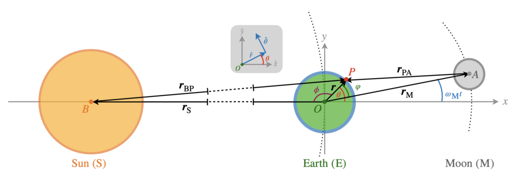
We will approach the problem as follows: we will first construct the gravitational potential at an arbitrary point P on the equator due to the moon and the sun. From the potential, we can then compute tidal forces and corresponding elevation of the water surface. Note that the point P has position vector \boldsymbol{r} relative to the origin O. Due to the circular symmetry, we will sometimes work in polar coordinates (r,\theta) instead of cartesian coordinates.

Potential due to Moon

Consider an element of mass m at point P, located at:

\begin{align*}
\boldsymbol{r}=r(\cos\theta\;\hat{x}+\sin\theta\;\hat{y}),
\end{align*}

i.e. at polar coordinates (r,\theta). Since we are at the equator, r is the radius of the earth by definition. We start by constructing the gravitational potential on this mass due to the moon, whose trajectory is given by:

\begin{align*}
\boldsymbol{r}_\mathrm{M}=r_M(\cos\omega_\mathrm{M}t\;\hat{x}+\sin\omega_\mathrm{M}t\;\hat{y}).
\end{align*}

and will include the contribution of the sun to the total potential at P at a later stage. This possible because potentials are additive: to get the total potential at a point of interest we simply add the potentials of all contributing sources.

The position vector from the center of mass of the moon to P is \boldsymbol{r}_\mathrm{PA}, so that we get:

\begin{align*}
V_\mathrm{M}=-\frac{GmM_\mathrm{M}}{|\boldsymbol{r}_\mathrm{PA}|},
\end{align*}

where M_\mathrm{M} is the mass of the moon. The mass m of the element appears as a multiplicative factor in gravitational potentials, so it is customary to work with the potential per unit mass instead:

\begin{align*}
\Phi_\mathrm{M}=-\frac{GM_\mathrm{M}}{|\boldsymbol{r}_\mathrm{PA}|}.
\end{align*}

To rewrite the factor 1/|\boldsymbol{r}_\mathrm{PA}| consider the triangle OPA. The angle opposite of side PA is:

\begin{align*}
\varphi(t) = \theta - \omega_\mathrm{M} t,
\end{align*}

and we have \boldsymbol{r}_\mathrm{PA}=\boldsymbol{r}-\boldsymbol{r}_\mathrm{M} by construction. Taking the dot product of \boldsymbol{r}_\mathrm{PA} with itself, we get:

\begin{align*}
\boldsymbol{r}_\mathrm{PA}\cdot \boldsymbol{r}_\mathrm{PA}&=\boldsymbol{r}\cdot\boldsymbol{r}+\boldsymbol{r}_\mathrm{M}\cdot\boldsymbol{r}_\mathrm{M}-2\boldsymbol{r}\cdot\boldsymbol{r}_\mathrm{M} = r_\mathrm{M}^2\bigg[ 1+\frac{r^2}{r_\mathrm{M}^2}-2\frac{r}{r_\mathrm{M}}\cos\varphi \bigg].
\end{align*}

The potential at P due to the moon can then be written as:

\begin{align*}
\Phi_\mathrm{M}=-\frac{GM_\mathrm{M}}{r_\mathrm{M}} \bigg[ 1+\frac{r^2}{r_\mathrm{M}^2}-2\frac{r}{r_\mathrm{M}}\cos\varphi \bigg]^{-1/2}.
\end{align*}

The inverse square root can be written as a series of Legendre polynomials to obtain:

\Phi_\mathrm{M}=-\frac{GM_\mathrm{M}}{r_\mathrm{M}}\sum_{n=0}^\infty \bigg(\frac{r}{r_\mathrm{M}}\bigg)^n P_n(\cos\varphi)\equiv\sum_{n=0}^\infty\Phi_n,

where P_n(\cos\varphi) are the Legendre polynomials. Note that this a power series in the parameter \epsilon_\mathrm{M} \equiv r/r_\mathrm{M}\ll 1, the ratio of the earths radius and the lunar orbit radius. Therefore, the series converges rapidly and only retaining the lowest order terms gives an accurate approximation to the potential:

\begin{align*}
\Phi_\mathrm{M}=-\frac{GM_\mathrm{M}}{r_\mathrm{M}}\bigg[1+\epsilon_\mathrm{M}\cos(\varphi)+\frac{\epsilon_\mathrm{M}^2}{2}(3\cos^2\varphi-1)+\cdots\bigg]=\Phi_0+\Phi_1+\Phi_2+\cdots. 
\end{align*}

We can interpret the result as follows. The first term gives the potential due to the moon at the center of the earth O. The other terms, proportional to powers of \epsilon_\mathrm{M}, give small corrections that account for the fact that we actually compute the potential at P and not at the origin O.

Force due to Moon

To get some more physical insight, let us compute the force corresponding to the potential of the moon, via \boldsymbol{F}_\mathrm{M}=-m\nabla\Phi_\mathrm{M}. Without loss of generality, we calculate the force at t=0 so that \varphi=\theta and the moon is located on the positive x axis. The zeroth term in the series (\Phi_0) gives no force at all, since it does not depend on the coordinates. The first term gives:

\begin{align*}
\boldsymbol{F}_{1,\mathrm{M}} = -m\nabla\Phi_1 &= +\frac{GmM_\mathrm{M}}{r_\mathrm{M}^2}\cos\theta\;\hat{r} - \frac{GmM_\mathrm{M}}{r_\mathrm{M}^2}\sin\theta\;\hat{\theta}\\
&=+\frac{GmM_\mathrm{M}}{r_\mathrm{M}^2}\;\hat{x}=\frac{GmM_\mathrm{M}}{r_\mathrm{M}^2}\;\hat{r}_\mathrm{M},
\end{align*}

where we have transformed from polar to cartesian unit vectors after we calculated the gradient in polar coordinates using the following identities:

\begin{align*}
\hat{r}&=\cos\theta \;\hat{x}+\sin\theta \;\hat{y}\\
\hat{\theta}&=-\sin\theta\;\hat{x}+\cos\theta\;\hat{y}\\
\nabla &=\frac{\partial}{\partial r}\hat{r}+\frac{1}{r}\frac{\partial}{\partial \theta}\hat{\theta}. 
\end{align*}

The result \boldsymbol{F}_{1,\mathrm{M}} corresponds to the force the moon would exert on the mass element, were the mass element located at the centre of the earth. The second term (\Phi_2) provides a correction for the fact that we actually compute the potential at P rather than O. In other words, the second term is the primary correction quantifying the (small) difference in gravitational force the moon exerts on the center of the earth (O) and on the ocean-covered surface (P). It is this small correction that ultimately causes the tides, and therefore \Phi_2 is also called the tide-generating-potential.

Now, let us calculate the tidal force due to \Phi_2, via \boldsymbol{F}_\mathrm{2,M}=-m\nabla\Phi_\mathrm{2}. We take the same approach as before, but do not restrict ourselves to t=0, so that \varphi\neq\theta and \Phi_2=\Phi_2(r,\varphi). Fortunately, we have \partial \varphi/\partial\theta = 1 so that the gradient operator simply becomes:

\begin{align*}
\nabla &=\frac{\partial}{\partial r}\hat{r}+\frac{1}{r}\frac{\partial}{\partial \varphi}\hat{\theta}.
\end{align*}

After some transforming to cartesian coordinates and simplifying the result using some trigonometric identities, we get:

\begin{align*}
\boldsymbol{F}_{2,\mathrm{M}}&=\frac{GmM_\mathrm{M}}{r_\mathrm{M}^2}\epsilon_\mathrm{M}\big[-\cos\theta+3\cos\varphi\cos\omega t\big]\hat{x}\\
&+\frac{GmM_\mathrm{M}}{r_\mathrm{M}^2}\epsilon_\mathrm{M}\big[-\sin\theta+3\cos\varphi\sin\omega t\big]\hat{y}. 
\end{align*}

At t=0, this result is equivalent to Eqs. 5.54 in section 5.5 of Classical Dynamics of Systems and Particles by Thornton and Marion (in our notation). The expression above gives the tidal force exerted on the earth at point P by the moon.

Force due to Sun

The above calculation can be carried over to the case of the sun, which is actually much simpler, since we assume the sun to be stationary at \boldsymbol{r}_\mathrm{S}=-r_\mathrm{S}\hat{x}. Actually doing the computation is left as an exercise for the interested reader, the result for tidal potential due to the sun (\Phi_{2,\mathrm{S}}) is given by:

\begin{align*}
\Phi_{2,\mathrm{S}}=-\frac{GM_\mathrm{S}}{r_\mathrm{S}}\frac{\epsilon_\mathrm{S}^2}{2}(3\cos^2\phi-1),
\end{align*}

which is equivalent to the tidal potential of the moon upon replacing M_\mathrm{M}\to M_\mathrm{S},\;r_\mathrm{M}\to r_\mathrm{S},\;\epsilon_\mathrm{M}\to\epsilon_\mathrm{S}\equiv r/r_\mathrm{S} and \varphi\to \phi. Recognizing that \phi=\pi-\theta, we find that the tidal force due to the sun is:

\begin{align*}
\boldsymbol{F}_{2,\mathrm{S}} = \frac{2GmM_\mathrm{S}}{r_\mathrm{S}^2}\epsilon_\mathrm{S}\cos\theta\;\hat{x}-\frac{GmM_\mathrm{S}}{r_\mathrm{S}^2}\epsilon_\mathrm{S}\sin\theta\;\hat{y}.
\end{align*}

Ocean Elevation

Now we are in the position to calculate the elevation of the sea level at the point of interest P on the equator. We denote the elevation of the sea-level as h(t,\theta) and measure the elevation relative to the case in which the sun and moon would be absent, and only the earths gravity is at play. Under the combined gravitational force of the earth, moon and sun the sea level must be a surface of equal potential, called an equipotential, for otherwise the water would flow towards regions of lower potential.

We can compute h(t,\theta) as follows. Consider an element of water with mass m on the ocean surface (located on the equator). Due to the combined tidal force of the sun and the moon, the element of water will be elevated upwards by a distance h(t,\theta). The potential energy associated with the movement is mgh(\theta). Note that this potential energy must balance with tidal potential energy due to the sun an the moon:

\begin{align*}
V_\mathrm{T}(t,\theta)\equiv m\big[\Phi_{2,\mathrm{S}}(\theta)+\Phi_{2,\mathrm{M}}(t,\theta)\big],
\end{align*}

for otherwise it would not be an equipotential. That is, we must have:

\begin{align*}
mgh(t,\theta)+V_\mathrm{T}(t,\theta)=0.
\end{align*}

We can solve this equation for the elevation, yielding:

\begin{align*}
h(t,\theta)=h_\mathrm{M}\bigg[\frac{3}{2}\cos^2(\theta-\omega_\mathrm{M}t)-\frac{1}{2}\bigg]+h_\mathrm{S}\bigg[\frac{3}{2}\cos^2(\pi-\theta)-\frac{1}{2}\bigg],
\end{align*}

where the amplitudes are defined as:

h_\mathrm{M}\equiv \frac{M_\mathrm{M}r^4}{M_\mathrm{E}r_\mathrm{M}^3}=0.36\;\mathrm{m},\quad\quad\quad h_\mathrm{S}\equiv \frac{M_\mathrm{S}r^4}{M_\mathrm{E}r_\mathrm{S}^3}=0.18\;\mathrm{m}. 

This gives the elevation of the ocean-level at point P (at angle \theta) on the equator and time t.

But what about the rotation of the earth? An observer that is stationary with respect to the earth indeed makes one full revolution each day (T_\mathrm{R}=1\;\mathrm{day}), corresponding to \omega_\mathrm{R}=2\pi\;\mathrm{day}^{-1}. For a stationary observer on the equator starting at \theta=0, we simply have \theta=\omega_\mathrm{R}t. Such an observer is indicated by the red dot in the animation (top panel). The elevation measured by this observer is:

\begin{align*}
h(t)\equiv h(t,\omega_\mathrm{R}t)=h_\mathrm{M}\bigg[\frac{3}{2}\cos^2(\omega_\mathrm{R}t-\omega_\mathrm{M}t)-\frac{1}{2}\bigg]+h_\mathrm{S}\bigg[\frac{3}{2}\cos^2(\pi-\omega_\mathrm{R}t)-\frac{1}{2}\bigg],
\end{align*}

which is depicted in the lower left panel of the animation.

Connection to Real Tides

In the simulations, we have made a number of simplifying assumptions. However, the peak to peak excursion of the water level is about 0.54\;\mathrm{m}, which is the same order of magnitude as typical observed tides, see Tidal distortion: Earth tides and Roche Lobes by Hale Bradt, 2008. Compare our animation for instance to the measured tides in Bridgeport (Connecticut, USA) over a month. Not only the amplitude is comparable, but also the oscillatory profile encoding the spring and neap tides are recognizable. This shows the art of simplification: even by making a large number of simplifying assumptions and approximations, we still obtained a reasonably accurate model.

A Common Confusion: (Why) Are Tidal Bulges Symmetric?

In the simulations, you can see the generation of tidal bulges due to the gravitational effects of the sun and the moon. It may be rather surprising that these bulges seem to appear symmetrically on both sides of the earth. More specifically, consider the sole effect of the moon in the schematic below. The generation of a tidal bulge on the side of the earth facing the moon can be understood intuitively. However, the schematic suggests a symmetric bulge is also generated on the opposite side of the earth, as if the moon’s gravity ‘pushes the ocean away from the earth on that side’. Of course, this cannot be the case since gravity is attractive. What is actually going on?

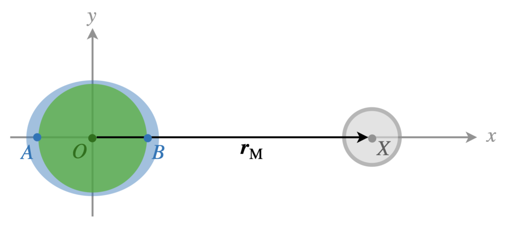
The (subtle) answer lies in the fact the earth is not fixed, but is actually in free-fall towards the moon. Consider the reference frame as indicated in the schematic. We will compute the gravitational acceleration (on a test mass) located at points A, O and B:

\begin{align*}
\boldsymbol{a}_A & =\frac{GM_E}{R_\mathrm{E}^2}\hat{x} + \frac{GM_\mathrm{M}}{(r_\mathrm{M}+R_\mathrm{E})^2}\hat{x} \\
\boldsymbol{a}_O & = \frac{GM_\mathrm{M}}{r_\mathrm{M}^2}\hat{x}\\
\boldsymbol{a}_B & = -\frac{GM_E}{R_\mathrm{E}^2}\hat{x} + \frac{GM_\mathrm{M}}{(r_\mathrm{M}-R_\mathrm{E})^2}\hat{x}
\end{align*}

Note that |\boldsymbol{a}_A|<|\boldsymbol{a}_O|<|\boldsymbol{a}_B|, which intuitively makes sense: the moon pulls strongest on B since it is closest to the moon and weakest on A. The moon pulls slightly harder on the ocean at B compared to the solid earth ( |\boldsymbol{a}_B|>|\boldsymbol{a}_O|), causing the bulge facing the moon. Similarly, the moon pulls slightly harder on the solid earth than on the ocean at A (|\boldsymbol{a}_A|<|\boldsymbol{a}_O|), effectively causing a tidal bulge on the side opposite of the moon as well.

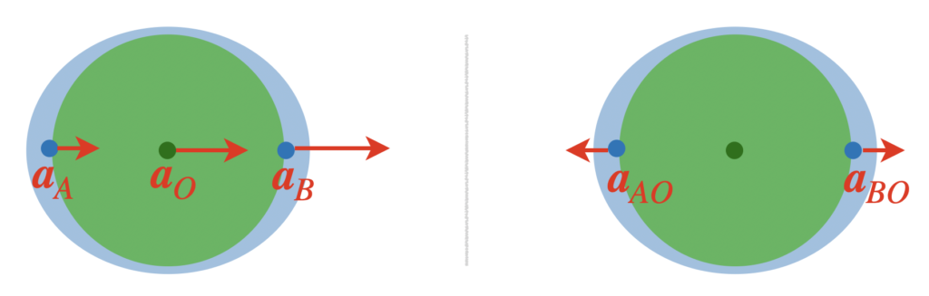
This explains why we get a tidal bulge at the face opposite to the moon, but not why the two bulges should be symmetric. After all, gravity scales as one over distance squared, so it would be logical to expect that the tidal bulge at A is smaller than at B. Why do they appear to have the same size? To answer this question, we look at the acceleration at A and B, relative to the center of the earth O by subtracting \boldsymbol{a}_O:

\begin{align*}
\boldsymbol{a}_{AO}=\boldsymbol{a}_A - \boldsymbol{a}_O& = \frac{GM_E}{R_\mathrm{E}^2}\hat{x} + \frac{GM_\mathrm{M}}{(r_\mathrm{M}+R_\mathrm{E})^2}\hat{x} -  \frac{GM_\mathrm{M}}{r_\mathrm{M}^2}\hat{x}  \\
\boldsymbol{a}_{BO}=\boldsymbol{a}_B - \boldsymbol{a}_O & = -\frac{GM_E}{R_\mathrm{E}^2}\hat{x} + \frac{GM_\mathrm{M}}{(r_\mathrm{M}-R_\mathrm{E})^2}\hat{x} -   \frac{GM_\mathrm{M}}{r_\mathrm{M}^2}\hat{x}
\end{align*}

To make further progress, we use the fact that the orbital radius is much smaller than the earths radius R_\mathrm{E}, so we can expand the fractions 1/(r_\mathrm{M}\pm R_\mathrm{E})^2 in \varepsilon \equiv R_\mathrm{E}/r_\mathrm{M}\ll 1:

\begin{align*}
\frac{1}{(r_\mathrm{M}\pm R_\mathrm{E})^2} = \frac{1}{r_\mathrm{M}^2}\Big(1\mp 2\varepsilon +\mathcal{O}(\varepsilon^2)\Big)
\end{align*}

Using this expansion, we obtain:

\begin{align*}
\boldsymbol{a}_{AO} & =\frac{GM_E}{R_\mathrm{E}^2}\hat{x} - \frac{GM_\mathrm{M}}{r_\mathrm{M}^2}\;2\varepsilon\;\hat{x} \\
\boldsymbol{a}_{BO} & = -\frac{GM_E}{R_\mathrm{E}^2}\hat{x} + \frac{GM_\mathrm{M}}{r_\mathrm{M}^2}\;2\varepsilon\;\hat{x}
\end{align*}

Notice that the these two accelerations are equal in magnitude but opposite in direction: \boldsymbol{a}_{AO}=-\boldsymbol{a}_{BO}. Relative to the solid earth, the ocean is pushed away from the earth equally strongly at both A and B. This explains why the tidal bulges are symmetric on both sides of the earth. However, beware that this result only hold up to first order in the parameter \varepsilon. At higher order, you would indeed find that the magnitude of \boldsymbol{a}_{AO} is slightly smaller than that of \boldsymbol{a}_{BO}, in line with intuition. The effect of higher order terms is however at the sub-percent level compared to the term linear in \varepsilon.

Downloads