Theoretical Context
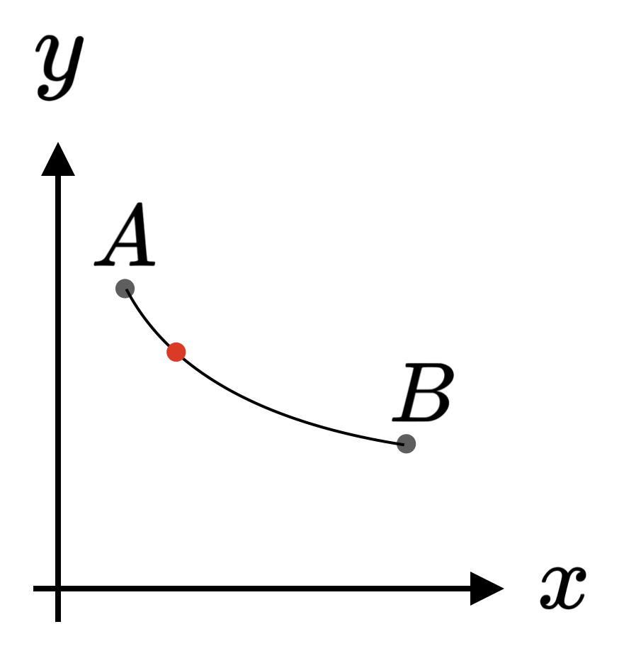
Consider a (red) bead on an frictionless wire between the points (x_A,y_A) and (x_B,y_B), see the schematic below. The wire is bend in an arbitrary shape described by the curve y=f(x). What shape minimizes the time it takes to get from A to B? The answer is the well-known brachistochrone curve. On this page, we want to visualize that this shape indeed minimizes the travel time via an animation making an explicit comparison to other well known shapes.
Lagrangian Approach
This problem can be treated within the Newtonian formulation of classical mechanics as will be shown in the next section. However, given the fact that it deals with constrained motion, using the Lagrangian formalism is way more convenient. Since we ignore friction, the only form of potential energy is gravitational potential energy and the Lagrangian for a bead of mass m can be written as:
\begin{equation*}
L=K-V=\frac{1}{2}m(\dot{x}^2+\dot{y}^2)-mgy.
\end{equation*}
However, note that x and y are not independent, since the wire enforces y=f(x). In the Newtonian formalism, this would result in a constraint force (read normal force) exerted by the wire on the bead. How do those constraints appear in the Lagrangian formalism? Answer: via so-called Lagrange multipliers \lambda. These Lagrange multipliers are treated as coordinates within the Lagrangian, i.e. on the same footing as the regular coordinates (in this case x,y).
In the spirit of the current example, we consider the case with only one constraint below, but we could generalize to multiple constraints. The constraint is written in the form:
h(x,y)\equiv 0,
such that in our case we have h(x,y)=y-f(x). To include the constraint, we define a new Lagrangian by adding the product of the multiplier and the constraint:
\begin{align*}
L'(x,y) &=L(x,y)+\lambda \;h(x,y)\\
&=\frac{1}{2}m(\dot{x}^2+\dot{y}^2)-mgy+\lambda h(x,y).
\end{align*}
Recall that we treat \lambda as a new coordinate. Since L' does not depend on \dot{\lambda}, the equation of motion for the multiplier is:
\begin{align*}
\frac{\partial L'}{\partial\lambda}=h(x,y)=0,
\end{align*}
which gives us back the constraint. The equations for the coordinates q=x,y are given by:
\frac{d}{dt}\bigg(\frac{\partial L'}{\partial \dot{q}}\bigg)-\frac{\partial L'}{\partial q}=\lambda\frac{\partial h}{\partial q}. The left-hand-side given the equation of motion were the constraints absent. The right-hand-side defines the constraint forces in the system, analogous to the introduction of the normal force in the Newtonian treatment. Defining \lambda_m\equiv \lambda/m, the resulting equations of motion are:
\begin{align*}
\ddot{x}&=-\lambda_m f'(x),\\
\ddot{y}&=-g+\lambda_m,
\end{align*}
where a prime indicates a derivative with respect to x.
At this point, we still have three unknown coordinates and will proceed as follows. We seek a differential equation for x(t) only, independent of the other two coordinates y,\lambda_m. Once we solve for this coordinate, we find y(t) via the constraint. To solve for x, we need to eliminate the Lagrange multiplier from the first equation above. We will do so by using the second equation. We want an expression for the Lagrange multiplier independent of y, for otherwise the differential equation for x would become dependent on y after substituting \lambda_m. Therefore, we have to eliminate \ddot{y} from the second equation, which can be done using the constraint:
\begin{align*}
\ddot{y}=f''\dot{x}^2+f'\ddot{x}.
\end{align*}
Using this relation and solving for the multiplier gives:
\begin{align*}
\lambda_m=\tau(f''\dot{x}^2+g),\quad\quad\quad\tau\equiv(1+f'^2)^{-1}.
\end{align*}
so that the differential equation for x reads:
\ddot{x}=-\tau f'(f''\dot{x}^2+g). For an arbitrary curve f(x) between the endpoints A and B, the above equation of motion can be solved numerically.
Newtonian Approach
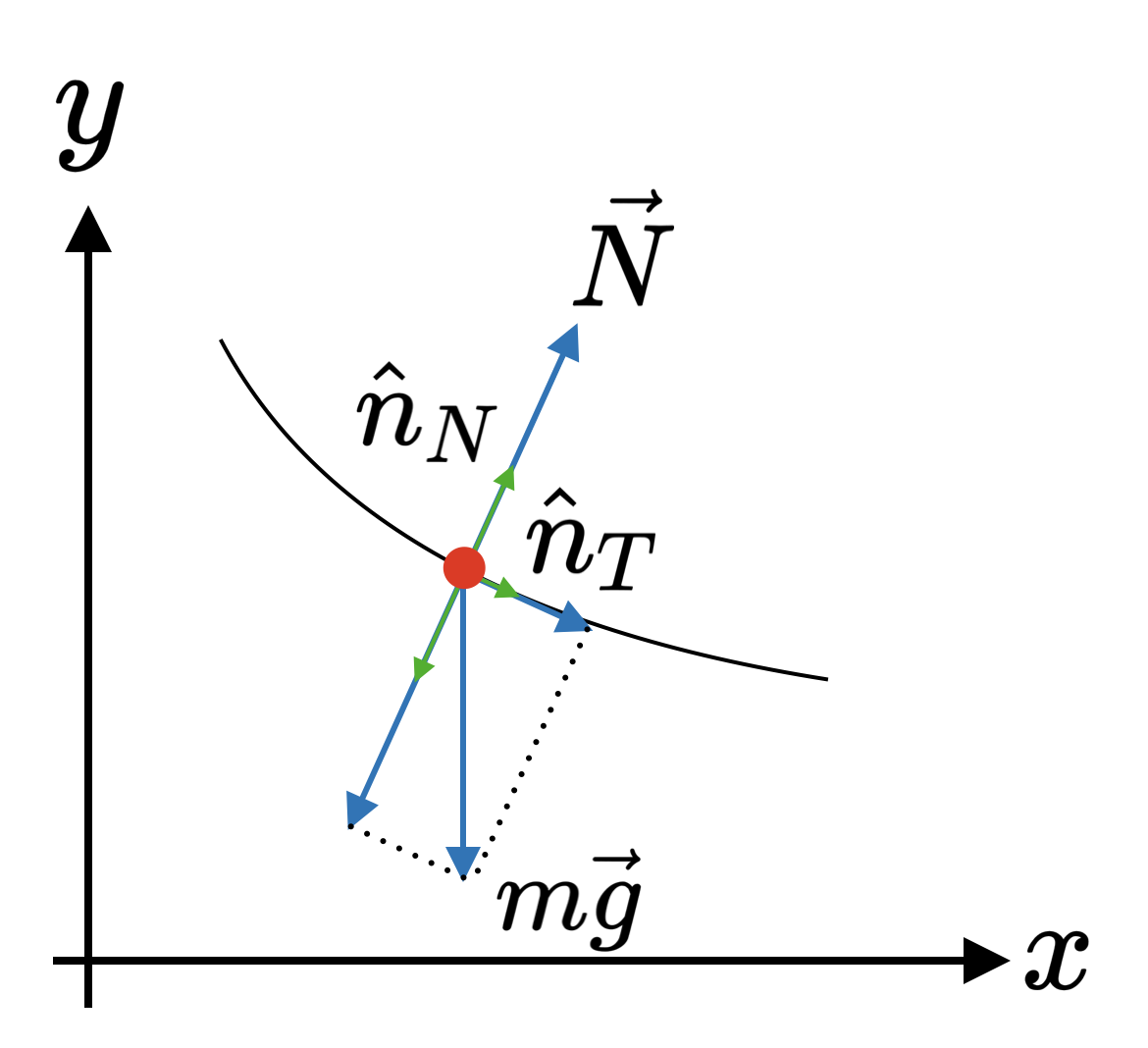
In the Newtonian approach, the component of the gravitational force normal to the curve is cancelled by the normal force, for otherwise the bead would not be constrained to move along the wire. The normal and tangential unit vectors can be constructed form the position vector of the bead:
\begin{align*}
\boldsymbol{r}=x\hat{x}+y\hat{y}=x\hat{x}+f(x)\hat{y}
\end{align*}
The derivative of the position vector with respect to x and its magnitude are given by:
\begin{align*}
\boldsymbol{r}'=\hat{x}+f'(x)\hat{y},\quad\quad\quad |\boldsymbol{r}'|=\sqrt{1+f'(x)^2}.
\end{align*}
The tangential and normal unit vectors are then:
\begin{align*}
\hat{n}_T=\frac{\boldsymbol{r}'}{|\boldsymbol{r}'|}=\frac{\hat{x}+f'(x)\hat{y}}{\sqrt{1+f'(x)^2}},\quad\quad\quad \hat{n}_N=\frac{\hat{n}_T'}{|\hat{n}_T'|}=\frac{\hat{y}-f'(x)\hat{x}}{\sqrt{1+f'(x)^2}}.
\end{align*}
Now we hare in the position to derive the equations of motion. Newton’s second law dictates that:
\begin{align*}
m\boldsymbol{a}=-mg\hat{y}+\boldsymbol{N}.
\end{align*}
Note that the normal force has to cancel the component of the gravitational force normal to the curve at every point. In other words, the magnitude of normal force is the projection of the gravitational force along -\hat{n}_T:
\begin{align*}
|\boldsymbol{N}|=(-mg\hat{y})\cdot(-\hat{n}_N)=\frac{mg}{\sqrt{1+f'(x)^2}},
\end{align*}
and the direction is +\hat{n}_N so that we have:
\begin{align*}
\boldsymbol{N}=\frac{mg}{1+f'(x)^2}\big[\hat{y}-f'(x)\hat{x}\big].
\end{align*}
Plugging this into the equation of motion we get:
\begin{align*}
\ddot{x}=-g\tau f'(x),\quad\quad\quad \ddot{y}=g(\tau-1).
\end{align*}
To show that this is identical to those equations are identical to the ones obtained in the Lagrangian approach, we have to perform some algebraic manipulations. We use the first equation to eliminate \tau from the second equation and eliminate \ddot{y} in the second using the constraint:
\begin{align*}
\ddot{y}&=-\frac{\ddot{x}}{f'(x)}-g\\
\ddot{x}&=-f'(x)\big[\ddot{y}+g\big]=-f'(x)\big[f'(x)\ddot{x}+f''(x)\dot{x}^2+g\big]\\
\ddot{x}&=-\tau f'(x)\big[f''(x)\dot{x}^2+g\big],
\end{align*}
which is indeed the same equation of motion as obtained in the Lagrangian approach, after some tedious algebra. It should be noted that, from a strict mathematical point of view there is nothing ‘special’ about this particular form of the equation of motion for x. However, it turns out that this form is well suited for numerical integration.
Travel Time
In the simulation, we consider a few different curves f(x). The time T it takes to complete each curve from A to B can be (numerically) calculated as:
\begin{align*}
T=\int_A^B \frac{ds}{v}=\int_{x_A}^{x_B} dx \sqrt{\frac{1+f'(x)^2}{-2gf(x)}}.
\end{align*}
The numerator is simply ds=\sqrt{dx^2+dy^2}=dx\sqrt{1+f'(x)} and the denominator follows from energy conservation. We define the point A to be at zero potential energy. The kinetic energy of the bead at A is zero, so that energy conservation dictates that E=0. Generically speaking, we have at any location x along the bead:
\begin{align*}
E(x)=\frac{1}{2}mv^2(x)+mgf(x)=0,\quad\quad\quad v(x)=\sqrt{-2gf(x)}.
\end{align*}
Curves
In the simulation, we take A to be at (0,0) and B at (1,-0.4). We consider three different shapes:
Linear. The first shape is a simple linear curve from A to B corresponding to f(x)=y_B\;(x/x_B).
Quadratic. We take a parabola with the minimum located at B, then f(x)=-y_B\;(x/x_B)^2+2y_B\;(x/x_B).
Brachistrochrone. The brachistochrone curve is characterized parametrically via:
\begin{align*}
x(\varphi)&=r(\varphi-\sin\varphi)\\
y(\varphi)&=r(\cos\varphi-1),
\end{align*}
where \varphi\in [0,\varphi_B] is the parameter. To find the value of the parameter at B, we divide the two equation to obtain:
\begin{align*}
\frac{y_B}{x_B}=\frac{1-\cos\varphi_B}{\varphi_B-\sin\varphi_B},
\end{align*}
and solve this implicit equation numerically for \varphi_B. Next, we can solve for r via:
\begin{align*}
r=\frac{y_B}{\cos\varphi_B-1}.
\end{align*}
Finally, we wish to relate the parameter \varphi to time. We set t=0 at point A. The total time it takes to complete the curve is:
\begin{align*}
T=\sqrt{\frac{r}{g}}\varphi_B.
\end{align*}
Since the parameter and time are linearly related, we therefore find that \varphi(t)=\omega t with \omega\equiv\sqrt{g/r}.
Simulation
Note that the brachistochrone curve, which minimizes the travel time between A and B, is solved analytically: we have the trajectory as a function time. The same can be done for the linear case. However, for the parabola it becomes more difficult already. Therefore the code attached below solves the problem numerically. In principle, the code should work for any well-behaved curve between A and B.