Bayesian Parameter Estimation – Physics Demonstrations

Theoretical Context

In Bayesian method of parameter estimation, the unknown parameter $\theta$ is treated as a random variable. To the parameter $\theta$ , a prior distribution $f_\Theta(\theta)$ is assigned, which encodes what we know about the parameter before observing the data. For a given value $\Theta=\theta$ , the data have a probability density function $f_{X|\Theta}(x|\theta)$ . In this notation, read $X|\Theta$ as the (probability of) $X$ given $\Theta$ . The joint distribution of $X$ and $\Theta$ can then be written as:

\begin{equation*} f_{X,\Theta}(x,\theta)=f_{X|\Theta}(x|\theta)\;f_\Theta(\theta). \end{equation*}

Joint Distribution: the probability density function $f_{A,B}(a,b)$ is defined such that $f_{A,B}(a,b)\;da\;db$ gives the probability that $a\leq A\leq a+da\wedge b\leq B\leq b+db$ .

The marginal distribution of the data is obtained, by definition, upon integrating over the parameter space:

\begin{equation*} f_X(x)=\int d\theta\;f_{X,\Theta}(x|\theta)=\int d\theta \;f_{X|\Theta}(x|\theta)\;f_\Theta(\theta). \end{equation*}

However, note that we can also write the joint distribution as $f_{X,\Theta}(x,\theta)=f_{\Theta|X}(\theta|x)\;f_X(x)$ , so that the distribution of $\Theta$ given the data $X$ is given by:

\begin{equation*} f_{\Theta|X}(\theta|x)=\frac{f_{X,\Theta}(x,\theta)}{f_X(x)}=\frac{f_{X,\Theta}(x,\theta)f_\Theta(\theta)}{\int d\theta\;f_{X,\Theta}(x,\theta)f_\Theta(\theta)}. \end{equation*}

This is also called the posterior distribution, representing what we know about $\Theta$ given the data $X$ . The denominator serves as a normalization constant. The information is contained in the numerator:

\begin{equation*} \mathrm{posterior\;density}\propto\mathrm{likelihood}\times\mathrm{prior\;density}. \end{equation*}

To construct the Bayesian estimate $\hat{\theta}_{\mathrm{Bay}}$ , we can extract the average or most probable value from the posterior distribution: this is a mere choice. As a measure for the variance of the estimate, we can take the standard deviation of the distribution.

Example

Let us consider the exponential distribution again, so that $f_{X_i|\Lambda}(x_i|\lambda)=\lambda e^{-\lambda x_i}$ . The conditional distribution $f_{X|\Lambda}(x|\lambda)$ is then given by:

\begin{equation*} f_{X|\Lambda}(x|\lambda)=\prod_{i=1}^n\lambda e^{-\lambda x_i}=(\lambda e^{-\lambda\bar{x}_n})^n, \end{equation*}

where $\bar{x}_n$ is the sample average for the sample of size $n$ .

There is no formal prescription for what the prior distribution should look like. Usually, we take a conservative approach that is as unbiased as possible, so that the data can speak for themselves. To this end, we take a flat prior, that is constant on a interval in which we expect the true parameter to be. Assuming the parameter to fall inside the interval $\lambda\in[\lambda_\mathrm{min},\lambda_\mathrm{min}]$ , we get:

\begin{equation*} f_\Lambda(\lambda)=\frac{1}{\lambda_\mathrm{max}-\lambda_\mathrm{min}},\quad\quad\quad \lambda_\mathrm{min}\leq\lambda\leq\lambda_\mathrm{max}, \end{equation*}

and zero otherwise. Ofcourse, choosing the interval to be very narrow makes even a flat prior biased. We will take the most conservative approach; we only assume that the parameter is positive and take the interval $\lambda\in[0,\infty)$ . The posterior is then:

\begin{equation*} f_{\Lambda|X}(\lambda|x)=\frac{(\lambda e^{-\lambda \bar{x}_n})^n}{I(x)},\quad\quad\quad I(x)\equiv \int_{0}^{\infty}d\lambda \; (\lambda e^{-\lambda \bar{x}_n})^n, \end{equation*}

where $I(x)$ is a normalization factor depending on the data. Notice that since the prior is flat, it cancelled out of the posterior: the only traces it left are the integration bounds on the normalization integral. The normalization integral can be written in terms of the gamma function as:

\begin{equation*} I(x)=\frac{1}{(\bar{x}_nn)^{n+1}}\int_0^\infty dy\; y^n e^{-y} = \frac{\Gamma(n+1)}{(\bar{x}_nn)^{n+1}}. \end{equation*}

Therefore, we find the posterior to be:

\begin{equation*} f_{\Lambda|X}(\lambda|x)=\frac{(\bar{x}_nn)^{n+1}}{\Gamma(n+1)}(\lambda e^{-\lambda \bar{x}_n})^n, \end{equation*}

which can be recognized as a Gamma distribution $f(\lambda;\alpha,\beta)=\beta^\alpha\lambda^{\alpha-1} e^{-\beta\lambda}/\Gamma(\alpha)$ with parameters $\alpha=n+1$ and $\beta=n\bar{x}_n$ . From the posterior, we take the expectation value as the estimate and the standard deviation as the error in the estimate:

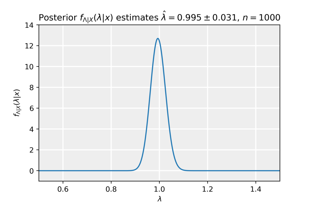
\begin{equation*} \hat{\lambda}_{\mathrm{Bay}}=\mathbb{E}[\lambda]=\frac{\alpha}{\beta}=\frac{n+1}{n\bar{x}},\quad\quad\quad\sigma^2_{\hat{\lambda}}=\mathbb{E}[\lambda^2]=\frac{\alpha}{\beta^2}=\frac{n+1}{n^2\bar{x}^2}. \end{equation*}

In the limit of large sample size $n\to\infty$ , we find that the estimator becomes $\hat{\lambda}_{\mathrm{Bay}}=1/\bar{x}$ , equivalent to the Method of Moments and Maximum Likelihood Method estimators, the same applies to the error estimates. Below, we plot the posterior obtained for a sample of size $n=1000$ , together with the estimate and its error.

Posterior distribution for estimation of parameter $\lambda$ .

Downloads

BayesINFER.Ipynb