Central Limit Theorem

Theoretical Context

Let \{X_1,X_2,\dots,X_n\} be a sequence of n independent identically distributed (i.i.d.) random variables drawn from a distribution with expected value \mathrm{E}[X_i]=\mu and variance \mathrm{Var}[X_i]=\sigma^2. The sample average is defined as:

\begin{equation*}
\bar{X}_n=\frac{1}{n}\sum_{i=1}^n X_i,
\end{equation*}

which itself is a random variable. The central limit theorem states the following:

Central Limit Theorem: As the sample size approaches infinity, n\to\infty, the distribution of the random variable \sqrt{n}(\bar{X}_n-\mu) converges to a normal distribution \mathcal{N}(0,\sigma^2).

In the above, the notation \mathcal{N}(\mu,\sigma^2) means a normal or Gaussian distribution with expected value or average \mu and variance \sigma^2.

Practical Meaning

In practice, the CLT implies the following. Suppose we draw a sample of n i.i.d. random variables \{x_1,x_2,\dots,x_n\} from some distribution with true mean \mu and variance \sigma^2, which need not be normal. We compute the sample average \bar{x}. We repeat this procedure m times, which results in a sequence of sample averages \{\bar{x}_1,\bar{x}_2,\dots,\bar{x}_m\}. The CLT states that, as the sample size n becomes sufficiently large, the distribution of the rescaled variables \sqrt{n}(\bar{x}_i-\mu) approaches that of a normal distribution with zero mean and variance \sigma^2. Equivalently, the distribution of the sample averages \bar{x}_i approaches a normal distribution with average \mu and variance \sigma^2/n.

Note that the CLT is a deep and non-trivial statement: even if the underlying distribution is far from normal (e.g. Poisson, exponential or log-normal), then still the distribution of the averages will tend to a normal distribution. Proving the CLT is beyond the scope of this page. Instead, we will demonstrate the CLT by means of simulations in Python.

Proof of Principle

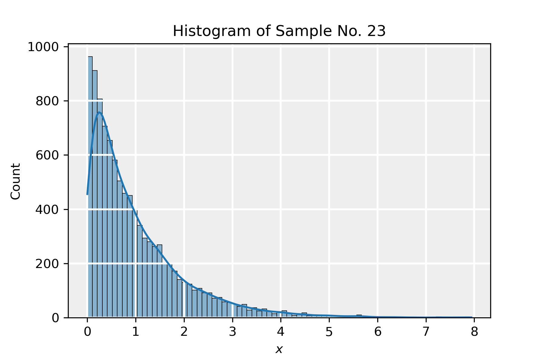
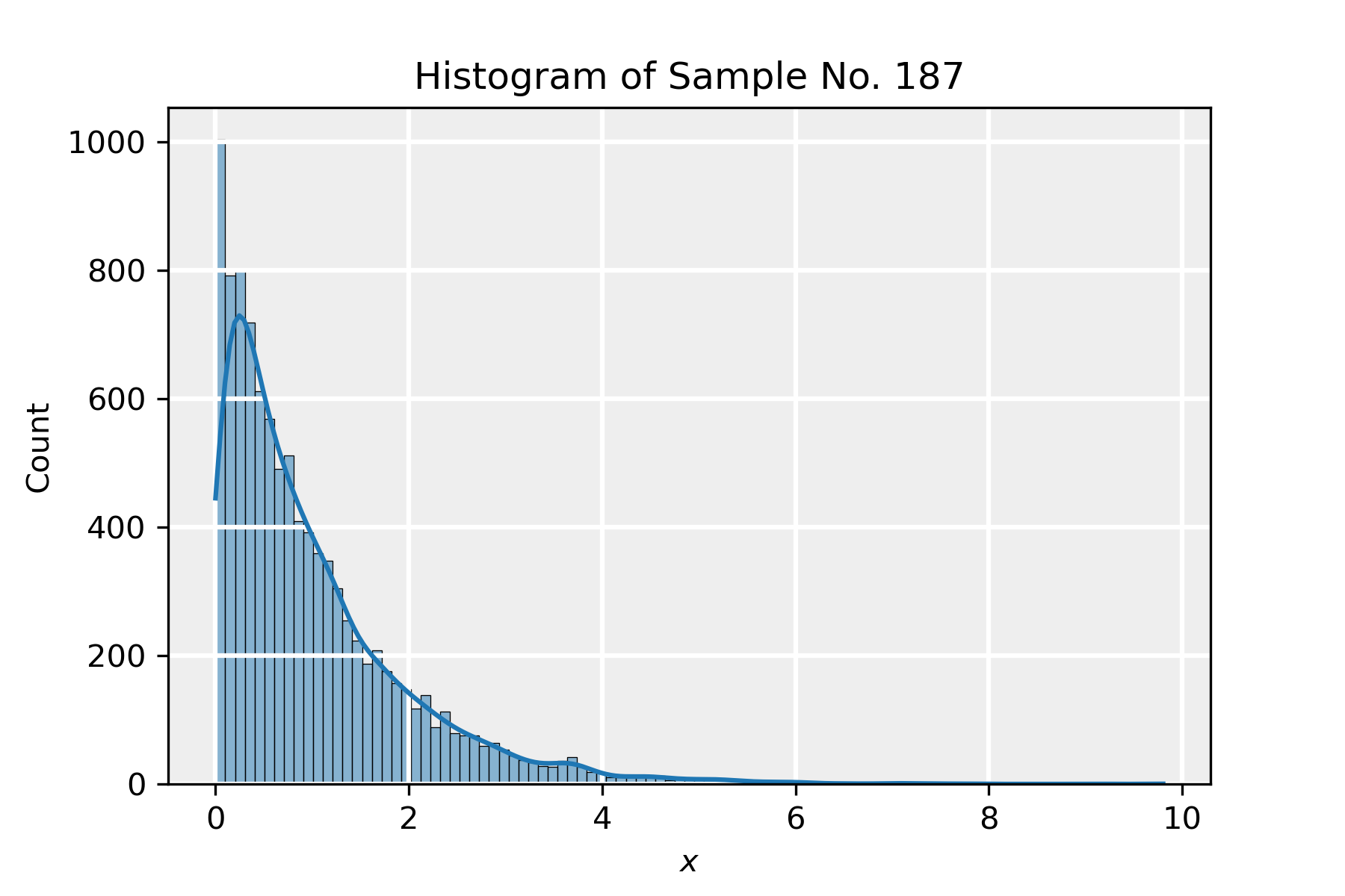
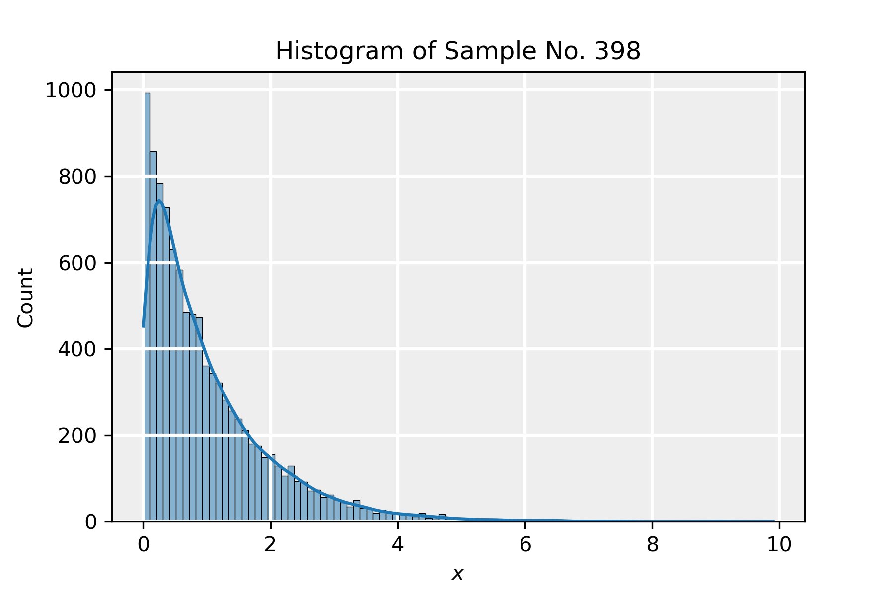
In the attached python notebook, we demonstrate the central limit theorem by taking a large number of samples drawn from an exponential distribution (which is very different in shape from a normal one) and show that the central limit theorem still applies to the distribution of the means of the samples.

The PDF of the exponential distribution is given by:

\begin{equation*}
f(x)=\begin{cases} \lambda e^{-\lambda x} &\mathrm{for }\; x \geq 0 \\
0 & \mathrm{for }\; x <0 \end{cases},
\end{equation*}

where \lambda>0 is the rate parameter of the distribution. The true mean is given by \mu=1/\lambda and the variance is given by \sigma^2=1/\lambda^2.

To demonstrate the central limit theorem, we proceed as follows:

1. We define the sample size n and the number of samples to be drawn from the distribution m.
2. We define a list that will contain the average of the samples.
3. We draw a sample of size n from the exponential distribution. We take \lambda=1 so that \mu=\sigma=1.
4. We compute the average of the sample \bar{x}_i, and store it in the list defined in step 2.
5. We repeat steps 3. and 4. m times.
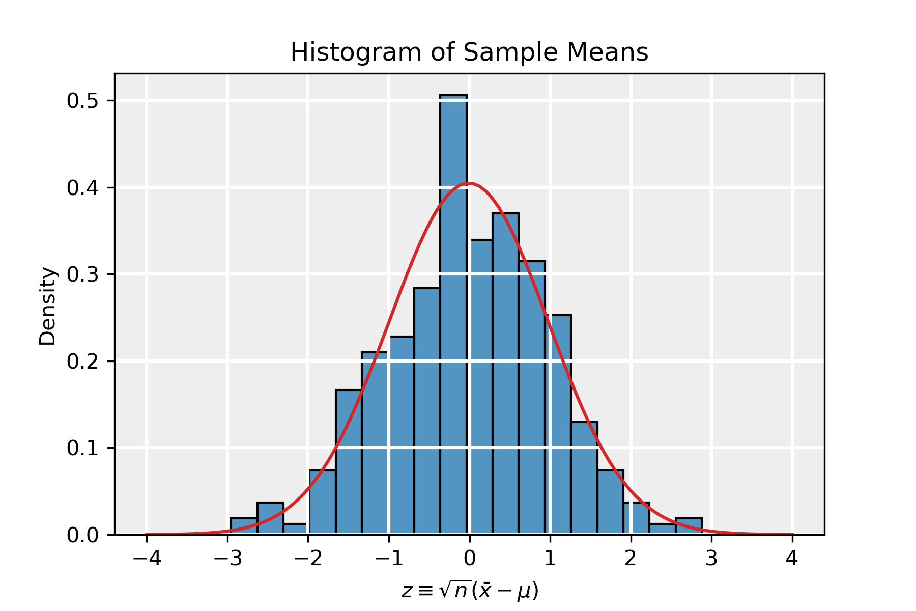
6. We finally produce a histogram of the rescaled data \sqrt{n}(\bar{x}_i-\mu). This should tend to a normal distribution with \mu=0 and \sigma^2=1.

In the slideshow below, we present the results of a simulation in which we took n=100 and m=10000. We present the histograms corresponding to four samples in the sequence and lastly show the distribution of the means of all the samples, in the form of the rescaled variable z\equiv \sqrt{n}(\bar{x}-\mu), which indeed tends to a normal distribution. The red PDF corresponds to a normal distribution with parameters \hat{\mu}=-0.0098 and \hat{\sigma}=0.98, which is in agreement with the distribution \mathcal{N}(0,1) as dictated by the CLT.

Test for Normality

The last figure in the slideshow shows the distribution of the average of the samples, which clearly follows a normal distribution to the eye. To make this statement more quantitative, we assess the skewness g_1 and (excess) kurtosis g_2. For a normal distribution, both of these identically vanish. We estimate the skewness and kurtosis, denoted by \hat{g}_1,\hat{g}_2, by using the moments. The r-th moment is extracted from a sample \{x_1,x_2,\dots,x_n\} via:

\begin{equation*}
m_r=\frac{1}{n}\sum_{i=1}^n (x_i-\bar{x})^r,
\end{equation*}

where \bar{x} is the sample average. The estimates for the skewness and kurtosis are then:

\begin{equation*}
\hat{g}_1=\frac{m_3}{m_2^{3/2}},\quad\quad\quad \hat{g}_2=\frac{m_4}{m_2^2}-3. 
\end{equation*}

Those estimates where found to be \hat{g}_1=-0.12\pm0.11 and \hat{g}_2=0.020\pm0.010, which are in agreement with the assumption of normality.

Downloads